One of my close friends runs an advisory for HS students applying to college. He wrote this guest post years ago: Moneyballing College Admissions.
He lives in the Bay Area and told me he’s seeing more parents complaining about the lack of acceleration options in the public school. He said outside CA it’s becoming far more common for high schoolers to take AP Calculus BC before senior year. My 8th graders’ goal is to take it by junior year, giving himself a chance to take Multivariate Calculus by senior year at a local college. This is already offered in some high schools across the nation, including some on the peninsula. Just this week, I talked to someone whose 9th grader was in Calc BC. That only sounds crazy if you haven’t been paying attention to what I’ve been sharing about Math Academy students (my 8th grader says his 5th grade little bro is already doing the same stuff his “advanced” math class is doing.)
In our local school district, we are finally seeing the pendulum swing the other way on math instruction. A few years ago, they got rid of “tracking” in 6th grade, forcing all kids, regardless of their interest/aptitude, into the same class. Well, the seeds of change are obvious in this survey I just filled out, as I don’t think we could have even had this conversation 5 years ago:
That #7 offers choices besides “supportive” and “very supportive” tells me these 2 articles are as important as I think they are.
Pamela Hobart argues “the academic acceleration community needs a viable brand”. Co-sign. Terrific post. I’ve had many of the same thoughts, especially as my kid’s schoolwork will leave me wondering, as Pamela has, “what are we even doing here?”
Everyone Wants a Child Like Eileen Gu (10 min read)
”almost nobody today wants the childhood that produced her.”
Violet Gordeljevic spitting truth in this one. I’ll share a few excerpts that resonated with me. You should read it to see what lands or doesn’t for you.
On Discipline and Exceptionalism
“So when people say she sounds and talks so disciplined, and that she knows her own mind—well, yes. That is what a decade of being asked to do your best looks like from the outside.”
“Nobody arrives at exceptional by accident. It doesn’t turn up later as a nice surprise because the child was left alone and bored for long enough.”
On Passion and Competence
“Passion doesn’t usually come first and then get supported. Usually exposure comes first, then competence (from actually having gone through practice), and passion tends to arrive somewhere after that, because human beings mostly love the things they are good at.”
“What is important to understand is that she could not have fallen in love with skiing, or Mandarin, or Olympiad maths, if nobody had ever put her in front of these things…A child who is never introduced to numbers will not reveal unusual mathematical ability. A child who never sits at an instrument will not discover she has an ear.”
On Modern Parenting and “Full Schedules”
“We didn’t lighten the load at all. We drive our children to more things than any generation in history. We just stopped asking them to become good at any of it.”
“If we are honest, the schedule is full but the demand is zero. It’s honestly like we have swapped skill for entertainment.”
“Underneath every version of this conversation sits the same line: I don’t need my child to be exceptional, I just want them to be happy. … But being the parent who stretches a child—who asks for one more go, who expects them to learn to write something properly or figure out that math equation, who holds the line at six when she wants to quit ballet—doing this is harder and considerably less pleasant than being her friend.”
On Warmth, Adversity, and Long-Term Value
“Protecting a child from effort is not the same as protecting a child.”
“What separates people with more demanding childhoods from those with easy, low demand ones, isn’t how much or even what was asked. It’s rather whether the asking sat inside enough warmth to be survivable.”
“The choice was never between pressure and love. It was always meant to be both.”
And then my 2 favorite:
“I have met a great many people who regret being allowed to quit”
“The thing is, children are not good judges of what they will be glad to be good at at thirty.”
Stand at one spot on a curve, measure everything you can there, and use those measurements to guess the height somewhere else.
You’d do this when the curve is hard to compute everywhere but easy to measure at one point, or when you want to see what drives a change. A bond’s price is a familiar case: you know its yield and duration today and want to know what happens if rates move.
The guess is built in layers. Each layer uses one more thing you measured at the anchor. The first layer is a straight line. The second bends it. The third bends the bend. You stop when the layers stop mattering, or when you run out of measurements.
Worked example: guess x³ at x = 1.2 using only what you know at x = 1
The curve is y = x³. You are standing at x = 1. The true answer is 1.2³ = 1.728, but pretend you can’t compute it.
What you know at x = 1
Thing
How you get it
Value at x = 1
Height
x³
1
Slope
derivative, 3x²
3
How fast the slope changes
derivative of that, 6x
6
How fast that changes
derivative of that
6
Anything further
derivative of a constant
0
The walk. Destination minus start: 1.2 − 1 = 0.2. Call it h.
Layer 1: pretend the slope stays 3. Guess = height + slope × walk = 1 + 3 × 0.2 = 1.6. Off by 0.128.
Layer 2: the slope drifts. It goes up at 6 per unit, so over the walk it rises from 3 to 3 + 6 × 0.2 = 4.2. Use the average slope, 3.6, instead of 3. Guess = 1 + 3.6 × 0.2 = 1.72. Off by 0.008.
Written as a separate correction: the new piece is ½ × 6 × 0.2² = 0.12, added to the 1.6.
Layer 3: the drift rate drifts. Same move one level deeper. The correction is 6 × 0.2³ ÷ 6 = 0.008. Guess = 1.728. Off by exactly 0.
Layer 4 and beyond: the measurement is 0, so every further correction is 0.
The guess is now perfect at x = 1.2, and it’s perfect at every other x too. x³ only has three pieces of information in it. Use all three and you have rebuilt the function.
Try it at x = 3 (walk h = 2): 1 + 3(2) + 3(2)² + (2)³ = 1 + 6 + 12 + 8 = 27 = 3³. Still exact, even two units from the anchor.
Layer 1 is the tangent line. Layer 2 bends it into a parabola that hugs the curve near x = 1 but misses on both sides. Layer 3 (dashed) lies on top of the black x³ curve at every x, which is the whole point: for a polynomial, enough layers is exactly the function.
Why you divide by 2, then 6, then 24
Each layer’s measurement gets divided before it’s used: layer 1 by 1, layer 2 by 2, layer 3 by 6, layer 4 by 24. Those are 1!, 2!, 3!, 4!. Two ways to see why.
The averaging picture. Layer 2 used the average slope over the walk. The slope was a ramp going from 3 to 4.2, and the average of a ramp is halfway: that’s the ÷2. Layer 3 needs the average of something that grows like a parabola, and a parabola from zero spends most of the walk being small, so its average is only a third of its end value: another ÷3. Stack them: 2 × 3 = 6. One more level and the average of a cubic is a quarter: 2 × 3 × 4 = 24.
Check the parabola claim with numbers. Sample t² at t = 0.1, 0.2, …, 1.0: you get 0.01, 0.04, 0.09, 0.16, 0.25, 0.36, 0.49, 0.64, 0.81, 1.00. They add to 3.85, average 0.385, and with finer sampling it settles to ⅓.
The power-raising picture. Differentiating hⁿ gives n × hⁿ⁻¹: lowering a power by one multiplies by that power. So raising a power by one divides by it. To turn a constant measurement into a term in h³ you raise the power three times, paying ÷1, ÷2, ÷3 along the way. That product is 3! = 6.
Layer
Measurement (x³ at 1)
Divide by
Term
1
3
1
3h
2
6
2
3h²
3
6
6
h³
4
0
24
0
Worked example: ln x, where the corrections stop helping
Same game, anchor at x = 1. Height is ln 1 = 0. Slope is 1/x, so 1 at the anchor.
What you know at x = 1
Layer
Derivative
Value at 1
Divide by
Term
1
1/x
1
1
h
2
−1/x²
−1
2
−h²/2
3
2/x³
2
6
h³/3
4
−6/x⁴
−6
24
−h⁴/4
5
24/x⁵
24
120
h⁵/5
6
−120/x⁶
−120
720
−h⁶/6
The measurements never hit zero. They alternate sign and grow. So there is always another correction, forever. Whether the corrections help depends on how far you walk.
Short walk: x = 1.5, so h = 0.5. True value ln 1.5 = 0.4055.
Layers used
Guess
Gap
1
0.5
0.0945
2
0.375
0.0305
3
0.4167
0.0112
4
0.4010
0.0044
5
0.4073
0.0018
6
0.4047
0.0008
Each layer roughly halves the gap. Keep going and it heads to zero.
Long walk: x = 2.5, so h = 1.5. True value ln 2.5 = 0.9163.
Layers used
Guess
Gap
1
1.5
0.5837
2
0.375
0.5413
3
1.5
0.5837
4
0.2344
0.6819
5
1.7531
0.8368
6
−0.1453
1.0616
The gap gets worse. Each term is ±hᵏ/k, and with h = 1.5 the hᵏ grows faster than the k can shrink it: 1.5, 1.125, 1.125, 1.27, 1.52, 1.90, … The guess swings wider and wider around the truth.
Inside the band the colored curves pile onto the black one, each layer tighter than the last. Right of x = 2 they fan out: layer 3 shoots up, layer 4 dives, layer 5 shoots higher, layer 6 dives harder. Every extra layer swings further from ln x instead of closer.
The rule. For ln x about 1, the corrections help when |h| < 1 and hurt when |h| > 1. That distance, 1, is the radius of convergence. It’s set by where the function itself breaks: ln x blows up at x = 0, exactly one unit left of the anchor, and the series can’t reach further right than it can reach left.
x³ had no such limit because its corrections ran out before they could misbehave. That is the difference between a polynomial and everything else.
the curve you’re guessing; f(x) is its height at x
x³
x
“x”
the destination, any point on the horizontal axis
1.2
x₀
“x-nought”
the anchor, where you stood and took measurements
1
x − x₀
“the walk”
destination minus start, also written h
0.2
P
“the polynomial”
the guess; a polynomial because it’s a sum of powers of the walk
1 + 3h + 3h² + h³
n
“n”
how many layers you used; the highest power in the guess
3
Pₙ(x)
“P-n of x”
the guess using n layers, evaluated at x
P₃(1.2) = 1.728
k
“k”
the counter: which layer you’re on, running 0, 1, 2, … up to n
0, 1, 2, 3
Σₖ₌₀ⁿ
“sum from k = 0 to n”
add up the term for every k from 0 through n
four terms
f′, f″, f‴
“f-prime, double-prime, triple-prime”
first, second, third derivative: slope, rate of slope, rate of that
3x², 6x, 6
f⁽ᵏ⁾
“f-k”
the k-th derivative; f⁽⁰⁾ is f itself, f⁽¹⁾ is f′, and so on
f⁽²⁾ = 6x
f⁽ᵏ⁾(x₀)
“f-k at x-nought”
the k-th derivative evaluated at the anchor, a plain number
1, 3, 6, 6
k!
“k factorial”
1 × 2 × … × k, the divide-by column; 0! = 1
1, 1, 2, 6
(x − x₀)ᵏ
“the walk to the k”
the walk raised to the layer number
1, 0.2, 0.04, 0.008
f(x) − Pₙ(x)
“the gap”
true height minus guess
0
ξ
“xi” (Greek letter)
some unknown point between x₀ and x; used only in the error formula
somewhere in [1, 1.2]
So the k = 2 term of the sum is: take the second derivative (6x), evaluate at the anchor (6), divide by 2! (3), multiply by the walk squared (0.04). That’s 0.12, the layer-2 correction from the worked example.
How big is the gap? It’s controlled by the next measurement you didn’t use, taken somewhere along the walk:
f(x) − Pₙ(x) = f⁽ⁿ⁺¹⁾(ξ) / (n+1)! · (x − x₀)ⁿ⁺¹ for some ξ between x₀ and x
Read it as: the gap is small when the walk is short (the hⁿ⁺¹ is tiny), when the next derivative is tame, or when n is large enough that (n+1)! dominates. The gap is large when the walk is long and the higher derivatives are big, which is exactly what happened to ln x at x = 2.5.
Real-world uses
Four places you’ve met this without the name. Each is worked with numbers.
Bond prices: duration and convexity. A 10-year zero at a 4% yield is priced 100/1.04¹⁰ = 67.56. The anchor is 4%. The two measurements are duration (layer 1, slope) = 10/1.04 = 9.62 and convexity (layer 2) = 10 × 11/1.04² = 101.7.
Yield rises 1%, so the walk is 0.01:
Layers
Guess
True price
Gap
1 (duration only)
67.56 × (1 − 9.62 × 0.01) = 61.06
61.39
0.33
2 (add convexity)
61.06 + 67.56 × ½ × 101.7 × 0.01² = 61.40
61.39
0.01
Yield rises 3%, walk 0.03: duration alone says 48.07, convexity pulls it to 51.16, true is 50.83. The gap is 30 times larger than for the 1% move. That’s the long walk. Traders quote duration and convexity for exactly the reason your tool quotes delta and gamma.
How a calculator computes sin. There’s no sin key inside the chip; it sums the series about 0: x − x³/6 + x⁵/120 − x⁷/5040 + ….
sin(0.5): 0.5 − 0.0208 + 0.0003 = 0.4794. True value 0.4794. Three terms.
sin(3): 3 − 4.5 + 2.025 − 0.434 + 0.050 − 0.004 = 0.137. True value 0.141. Six terms and still off in the third decimal. The series converges everywhere, unlike ln x, but a long walk needs many more layers. Calculators dodge this by folding the input back to a small angle first, which is the “walk less” strategy.
Pendulum clocks. The textbook period T = 2π√(L/g) comes from replacing sin θ with θ, which is layer 1 of the sine series. The next layer says the true period is longer by a factor of about 1 + θ₀²/16, where θ₀ is the swing in radians.
Swing
θ₀ in radians
Correction
Period error if you ignore it
5°
0.087
1.0005
0.05%
20°
0.349
1.0076
0.8%
60°
1.047
1.069
7%
A clock built on layer 1 keeps time at small swings and drifts at big ones. Same story: the anchor is θ = 0 and the walk is the amplitude.
Compound growth. (1 + r)ⁿ about r = 0 is 1 + nr + n(n−1)r²/2 + …. For 5% over 10 years: layer 1 says 1.50, layer 2 says 1.50 + 45 × 0.0025 = 1.61, true is 1.63. Layer 1 alone is the “simple interest” mental shortcut, and the layer-2 term is exactly how much compounding beats it.
All four break the same way ln x did. Past some size of move the layers you kept stop describing the function, and the fix is either more layers, a shorter walk, or computing the real thing.
Quick reference
Recipe for any function about any anchor
Pick the anchor x₀. Compute the walk h = x − x₀.
Take derivatives of f until you have as many as you want, and evaluate each at x₀.
Divide the k-th one by k!, multiply by hᵏ.
Add them up. That’s the guess. The leftover is the gap.
If the derivatives hit zero, the guess becomes exact. If they don’t, check whether the terms are shrinking; if not, you walked too far.
The two examples side by side
x³ about 1
ln x about 1
Derivatives at anchor
1, 3, 6, 6, 0, 0, …
0, 1, −1, 2, −6, 24, …
k-th term
3h, 3h², h³, then 0
(−1)ᵏ⁺¹ hᵏ / k
Exact after
3 layers
never
Works for
every x
0 < x < 2 only
Why
polynomial: information runs out
ln x breaks at 0, one unit from the anchor
Factorials
k
k!
Average of tᵏ over [0, h]
1
1
h/2
2
2
h²/3
3
6
h³/4
4
24
h⁴/5
5
120
h⁵/6
Common series about 0, for reference
Function
Series
Converges for
eˣ
1 + x + x²/2 + x³/6 + …
all x
sin x
x − x³/6 + x⁵/120 − …
all x
cos x
1 − x²/2 + x⁴/24 − …
all x
1/(1−x)
1 + x + x² + x³ + …
|x| < 1
ln(1+x)
x − x²/2 + x³/3 − …
−1 < x ≤ 1
The last two have a radius because the function breaks at x = 1 or x = −1. The first three never break, so the series works everywhere even though it never terminates.
Key Insights
What
Why it matters
Anchor and walk
Everything is measured at one point; the guess only ever knows about that point
Layers = derivatives
Each derivative at the anchor buys one more correction; that is all the information you have
Divide by k!
Raising a power costs a division each time; averaging a ramp, parabola, cubic costs ÷2, ÷3, ÷4
Polynomials terminate
Derivatives hit zero, so finitely many layers rebuild the function exactly, everywhere
Radius of convergence
For everything else, past the distance to the nearest breakdown the layers make the guess worse
The gap formula
The error is the first term you dropped, evaluated somewhere on the walk
Everything below is derived from these definitions. They’re the raw material — average squared deviation for variance, average product of deviations for covariance. When a derivation feels stuck, come back here and plug in.
Variance — average squared deviation from the mean
Var(X) = E[(X− μ)2] μ = E[X]
Covariance — average product of deviations
Cov(X, Y) = E[(X− μX)(Y− μY)]
Sum of squared deviations (the un-averaged version)
SS = Σ (xi− μ)2Var = SSn
Variance is just SS divided by n (or n−1 for a sample). Same object, before you average.
The move in every derivation: plug into one of these, expand the square or product (pure algebra), apply E using linearity, then recognize the Var/Cov patterns that fall out. The computational forms below (E[X2] − (E[X])2, E[XY] −E[X]E[Y]) are results of doing this, not starting points.
The identities
Variance from the definition
Var(X) = E[(X− μ)2] = E[X2] − (E[X])2
Average of the squares minus the square of the average. Worth showing where that second form comes from, since every later grind reuses this exact collapse. Start from the deviation definition and expand the square:
1nΣ(xi−x)2 = 1nΣ(xi2− 2xix + x2)
Average term by term. The key is that x is a constant (already computed), so it pulls out of the sums:
Last term: (1/n)Σx2 = x2 = (E[X])2 (averaging a constant returns the constant)
Put them together — and notice the last term carries a coefficient of 1, not 2:
E[X2] − 2(E[X])2 + (E[X])2 = E[X2] − (E[X])2
The −2 and +1 combine to −1. That collapse — middle and last terms both becoming (E[X])2 and partially cancelling — is the same move behind every Var/Cov identity on this sheet.
Covariance from the definition
Cov(X, Y) = E[(X− μX)(Y− μY)] = E[XY] −E[X]E[Y]
Average of the products minus the product of the averages.
Here a and b are the amounts held of each asset. They’re portfolio weights when they sum to 1. Var(X+Y) above is just this formula with a = b = 1 — one unit of each, no weighting lever. The weights are what turn a raw sum into a portfolio.
Worked example. Two assets: σX = 20%, σY = 10%, ρ = 0.3. Equal weights a = b = 0.5.
Compare to the naive weighted-average vol, 0.5·20% + 0.5·10% = 15%. The cross term (with ρ < 1) is what pulls portfolio vol below the average of the two vols. That gap is the diversification benefit.
Variance of a difference (spread variance / pair-trading formula)
Var(X−Y) = Var(X) + Var(Y) − 2 ·Cov(X, Y)
Same as Var(X+Y) but cross term flips sign. When X and Y are highly correlated, spread variance is small — the math behind why pair trades work.
Bilinearity of covariance
Cov(X, A + B) = Cov(X, A) + Cov(X, B)
Same in the first slot by symmetry.
Where it’s used. This is the move that lets you compute an asset’s covariance with a whole portfolio without re-deriving anything. Say a portfolio P = 0.5A + 0.5B and you want how asset A co-moves with the portfolio it sits in:
Distribute across the sum, pull the weights out. That number — an asset’s covariance with its own portfolio — is its marginal contribution to portfolio risk, and it’s exactly what you FOIL out when you expand Var(w1X1 + … + wnXn) into the full covariance matrix. Bilinearity is the engine under every portfolio-variance calculation.
Variance of a binomial
Var(H) = np(1−p) where H = ΣXi
Derived in two steps, both from scratch.
Step 1 — variance of a single flip. One flip X is 1 with probability p, 0 with probability (1−p). Mean is E[X] = p. Plug into the squared-deviation definition — deviations are (1−p) for heads and (0−p) = −p for tails, each weighted by its probability:
Var(X) = p(1−p)2 + (1−p)p2
Factor out p(1−p): the bracket is (1−p) + p = 1, so
Var(X) = p(1−p)
(Peaks at p = 0.5, value 0.25 — the fair coin is the most uncertain, most variance per flip.)
Step 2 — n flips. Write H as a sum of n independent single flips, H = X1 + … + Xn. Variance of a sum adds the pairwise Cov terms, but independent flips have Cov(Xi, Xj) = 0, so every cross term drops. The n identical variances just add:
Var(H) = ΣVar(Xi) = n·p(1−p)
The np(1−p) isn’t handed to you — it falls out of one Bernoulli’s p(1−p) times n, because independence kills the covariances.
Standard deviation scaling
StDev(aX) = |a| ·StDev(X)
Correlation definition
ρ = Cov(X, Y)σX· σY
When ρ = 1: Cov(X, Y)2 = Var(X) · Var(Y).
The derivation recipe
Every identity in this neighborhood comes out of the same five moves. When you see a Var or Cov of something built from linear combinations of random variables, this is the procedure.
Plug into the definition. Use Var(Z) = E[Z2] − (E[Z])2 or Cov(X, Y) = E[XY] −E[X]E[Y] depending on what you’re computing.
Expand squares and products. Pure algebra on the random variables. FOIL out any binomials. No expectations yet.
Apply E using linearity. Distribute E across sums, pull constants out of expectations. This is the step that does the most work. Always handle linearity first when you have the chance — squaring is not linear, so you simplify E first and let the square wrap what’s left.
Group matching terms. Line up the things that share factors (a2 terms together, ab terms together, b2 terms together, etc.).
Factor and recognize. Pull out shared factors and spot the patterns: (E[X2] − (E[X])2) is Var(X), and (E[XY] −E[X]E[Y]) is Cov(X, Y).
The reason this recipe always closes: variances and covariances are quadratic in the underlying random variables, so expanding any square or product of linear combinations only generates more variances and covariances. Step 5 is recognition, not computation. There’s nowhere else for the algebra to land.
Two applications
Interview problem: E[H·T] for n coin flips
Flip a fair coin n = 100 times. H = heads, T = tails. Find E[H·T]. Worked slowly, because the one-line answer hides about six moves.
Step 1 — first reach, and why it fails. The instinct is E[H·T] = E[H] ·E[T] = 50 · 50 = 2,500. But splitting a product of expectations like that is only legal when the two variables are independent. Check the precondition: H + T = 100, so knowing H pins down T exactly. Not independent. The naive split is off by a correction.
Step 2 — name the correction. That correction is what covariance is. Rearranging Cov(X, Y) = E[XY] −E[X]E[Y]:
E[H·T] = E[H] ·E[T] + Cov(H, T)
Independent → Cov = 0 → naive split exact. Locked → Cov ≠ 0 → you need the term.
Step 3 — get the sign first.H + T = 100, so when H is above its mean, T is forced below. They move opposite, always. So Cov(H, T) is negative, and the true answer lands below 2,500.
Step 4 — compute Cov(H, T) via substitution. Since T = 100 −H, write Cov(H, T) = Cov(H, 100 −H) and split with bilinearity:
Cov(H, 100 −H) = Cov(H, 100) + Cov(H, −H)
First term is covariance with a constant → 0. Second term, pull out the −1 (scaling rule, ab = 1 · (−1) = −1):
= 0 −Cov(H, H) = −Var(H)
So Cov(H, T) = −Var(H). Now it’s earned, not asserted.
Step 5 — Var(H) is the binomial variance.H is the count of heads in n flips, so Var(H) = np(1−p) = 100 · 0.5 · 0.5 = 25.
Step 6 — land it.
E[H·T] = 2,500 − 25 = 2,475
Where n(n−1) comes from. Keep everything in symbols instead of plugging in. E[H] = np and E[T] = n(1−p), so E[H]·E[T] = n2p(1−p), and Var(H) = np(1−p). Then:
Why this is the instructive form. Weights are fixed (50/50) and both vols are fixed (σ). The only thing left moving is ρ. So the entire diversification effect is carried by the single factor (1 + ρ)/2 — a clean dial from 0 to 1 that multiplies the single-name variance. Sweep ρ and read what correlation actually does:
ρ
Var(P)
σP (vol)
vs. one stock
+1
σ2
σ
no benefit — identical names
+0.5
0.75σ2
0.87σ
13% vol cut
0
0.5σ2
0.71σ
29% vol cut (the √½ case)
−0.5
0.25σ2
0.5σ
half the vol
−1
0
0
risk fully cancels
The variance scales linearly in ρ, but the thing you feel — vol, σP = σ√((1+ρ)/2) — scales as the square root, so the first chunk of decorrelation buys more than the last. Going from ρ = 1 to ρ = 0.5 already takes 13% off your vol. You do not need negative correlation to diversify; anything below +1 helps. Negative correlation is just the strong form, and ρ = −1 is the perfect hedge where the two positions cancel outright.
The whole two-name diversification story lives in that (1 + ρ)/2 factor. Same vols, same weights, and correlation alone moves you from “no benefit” to “risk gone.”
Two-stock unequal-weight portfolio with equal variances σ2 and correlation ρ
Var(P) = σ2 [1 − 2w(1−w)(1−ρ)]
Diversification benefit is the product of a weight piece (2w(1−w), maxed at w = 0.5) and a correlation piece (1−ρ). Need both to get benefit. With equal variances, equal weighting is optimal — any tilt from 50/50 sacrifices diversification.
Now drop the equal-variance assumption. Keep σX2 and σY2 separate. Weights w and (1−w):
Var(P) = w2σX2 + (1−w)2σY2 + 2w(1−w)ρσXσY
Minimize over w. Var(P) is an upward parabola in w (positive coefficient on w2), so the critical point is the min. Differentiate term by term and set to zero:
2wσX2− 2(1−w)σY2 + 2(1−2w)ρσXσY = 0
Divide by 2, expand, collect the w terms on the left and constants on the right, factor w out:
w(σX2 + σY2− 2ρσXσY) = σY2− ρσXσY
w* = σY2− ρσXσYσX2 + σY2− 2ρσXσY
The denominator is Var(X−Y) — the spread variance from earlier. The numerator is σY2− Cov(X, Y).
The payoff — set ρ = 0 (independent names):
w* = σY2σX2 + σY2 = 1/σX21/σX2 + 1/σY2
That’s inverse-variance weighting: each asset’s weight is its inverse variance over the sum of inverse variances. The quieter asset gets more money. This is the result behind Kalman filters, weighted least squares, and meta-analysis — anywhere you optimally combine noisy estimates, you weight by precision (1/variance). It’s also the “optimal” cousin of the inverse-vol risk-parity heuristic, which ignores correlations.
Intuition — hold σX fixed at 20% (σX2 = 0.04), turn the σY knob:
σY
σY2
w* on X
0
0
0
10%
0.01
0.20
20%
0.04
0.50
40%
0.16
0.80
∞
∞
→ 1
X’s weight is driven by Y’s variance, not its own. The noisier the alternative, the more you pile into X. Three anchors: σY2 = 0 → w* = 0 (Y is riskless, hold only Y); σY2 = σX2 → w* = 0.5 (equal variances recover equal weighting); σY2 → ∞ → w* → 1 (Y is pure noise, flee into X). The cleanest limit: if σX2 = 0, then w* = 1 — a riskless X takes the whole book. Precision is just quietness, and you trust the quiet estimate more.
Three-variable portfolio variance → why the matrix shows up
Same Form A grind, one more variable. Expand (aX + bY + cZ)2, apply E, subtract the squared-mean term. Every squared term becomes a variance, every cross term a covariance:
n variance terms — one per asset (the ai2 Var pieces)
nC2 = n(n−1)/2 covariance pairs — one per distinct pair
Total = n + nC2. For n = 3: 3 + 3 = 6. For n = 100: 100 variances + 4,950 covariance pairs. The cross terms grow as n2, which is exactly why nobody writes portfolio variance longhand past n = 3 — you switch to the matrix form.
The double-sum / matrix form. Organize every term into a grid indexed by asset pairs. With weights wi and returns ri:
Var(P) = ΣiΣjwiwjCov(ri, rj) = w⊤Σw
Reading the double sum: the outer Σ over i and the inner Σ over j together form every ordered pair (i, j). For each pair you drop in one term, wiwjCov(ri, rj), and add them all up. For n = 3 that’s 3 × 3 = 9 cells:
X (j=1)
Y (j=2)
Z (j=3)
X (i=1)
a2Var(X)
ab Cov(X,Y)
ac Cov(X,Z)
Y (i=2)
ab Cov(X,Y)
b2Var(Y)
bc Cov(Y,Z)
Z (i=3)
ac Cov(X,Z)
bc Cov(Y,Z)
c2Var(Z)
Sum all nine cells and you get the six-term formula above. Two things to see:
Diagonal (i = j, shaded): Cov(ri, ri) = Var(ri), so the diagonal is the n variance terms.
Off-diagonal (i ≠ j): each unordered pair appears twice — cell (X,Y) and cell (Y,X) are identical — and those two copies are exactly where the factor of 2 on each covariance comes from. You never write the 2 by hand; the grid double-counts it for you.
So Σ is the covariance matrix: variances down the diagonal, covariances off it. w⊤Σw just says “sweep every cell of the grid, weight it, sum it.” The n + nC2 count is the matrix — diagonal plus (doubled) upper triangle. You’ve already discovered why the matrix form is inevitable; it’s just bookkeeping for the term explosion.
Figure — the double sum is the matrix: one sweep, three views
Figure — three forms of the same variance, and where the 2s go
Notation you’ll see in practice: w⊤Σw. You’ll run into this constantly in risk models, optimizers, and quant papers. It’s the same portfolio variance, packaged as a matrix operation. Reading it piece by piece:
w — the weight vector, weights stacked in a column.
w⊤ — “w transpose,” the same weights laid flat as a row. Transpose just tips a column over into a row.
Σ — the covariance matrix (the grid above). Watch out: this capital-sigma is the matrix, not a summation sign. Variances on the diagonal, covariances off it.
So w⊤Σw is row-of-weights × matrix × column-of-weights, which multiplies out to a single number — the portfolio variance. It’s identical to the double sum, and in a spreadsheet it’s literally =MMULT(MMULT(TRANSPOSE(w), Σ), w).
Why bother, when the double sum already shows everything? Three practical reasons, none of them “it’s more correct.” It doesn’t grow — three symbols whether n is 2 or 2,000, where the double sum for 500 names is 250,000 terms. It’s how software actually computes portfolio variance (one fast matrix op). And optimization only speaks matrix: the minimum-variance weights come out as Σ−11 normalized, and the inverse Σ−1 has no double-sum spelling. The two-asset inverse-variance weighting derived above is Σ−1 for n = 2 — the matrix form is how that generalizes. For understanding, the double sum is enough; this is the notation for doing things with it.
The ladder
Each rung is built from the one before it — the definition first, then the algebra of scaling and adding, then portfolios, then the jump to the matrix. Nothing is assumed that wasn’t derived earlier.
1. Variance as average squared deviation
2. Var(X) = E[X2] − (E[X])2 — from the definition
3. Cov(X, Y) = E[XY] −E[X]E[Y] — from the definition
4. Var(aX) = a2·Var(X)
5. Cov(aX, bY) = ab·Cov(X, Y)
6. Cov(X + c, Y) = Cov(X, Y) and Cov(X, c) = 0
7. Var(X + Y) = Var(X) + Var(Y) + 2·Cov(X, Y)
8. Var(aX + bY) — the full weighted-sum workhorse
9. Two-stock equal-weight portfolio variance → the (1+ρ)/2 diversification factor
14. Var(aX + bY + cZ) — three variables, and the n + nC2 term count
15. General n-asset portfolio variance — the w⊤Σw matrix form
Is this one lesson in a math course?
No. This would be roughly half a semester of a first probability course, or a full chapter and a half of a more applied stats book.
Rough mapping to a standard curriculum:
Variance from the definition, E[X2] identity: one lecture, plus a problem set
Covariance and the product identity: one lecture
Scaling rules, bilinearity, variance of a sum: one to two lectures
Portfolio variance, weighted sums, correlation: one lecture in the probability course, or the opening week of a finance/portfolio-theory course
Binomial variance, applications: another lecture or two
So this is the equivalent of maybe four to six lectures of material, plus the problem sets that go with them. The reason it feels like a lot is that this sheet does the whole pipeline — derivation, intuition, numerical examples, applications — for each piece, instead of showing a formula and moving on.
The trade-off is real: this is slower but produces durable understanding. A typical math course shows you Var(aX + bY) on day one, leaves the “why it’s that and not something else” fuzzy, and you pattern-match for the rest of the semester. Done this way, when σ2· (1+ρ)/2 turns up in a textbook two years later, you see the bilinearity FOIL behind it instead of recognizing a memorized formula.
I usually have a concrete plan in advance of writing, but today’s letter is totally spontaneous, other than knowing that something would be published. I wrote it all, but found myself stuck on a title. I hope it will make sense by the time you’re done.
So…one of my oldest friends, someone I consider family really, is enjoying a sabbatical year. He and his wife crashed with us for 10 days. It’s one of those slices of time that you know before it’s even over that you will have nostalgia for.
We didn’t do anything overly special, although it was a great catalyst to convene with the rest of our Bay Area college crew over the weekend. The week was something in between a staycation and just a far more elevated (ie joyful) routine. I would work during the day while they went on an excursion, but we’d make sure to go to the gym or at very least a walk together daily, and the evenings were filled with good food (his baked ziti is in contention for my electric chair meal which I don’t anticipate needing unless they start rounding up the dorks) and games (Scrabble and Decrypto mostly) with the whole family.
One of my favorite parts of it was to have them around in such an informal way, just like family crashing. The kids would hang around and be part of the discussion like these were the aunties and uncles they normally see. Everyone actually gets to know each other. My kids get to see that their dad’s friends are weird just like their dad is. It’s funny for them to see them process it, but I hope it models to them what friendship is, even if they do think we’re old aliens. I’m also happy to see my friends know my kids. To see their different personalities and for them to be more than just names.
Personally, the week has been so much fun, especially because my friend and I have always had a nerd bond. He’s much more educated and technical than I (this sabbatical very likely ends with him working for Jane Street or Waymo), so I also just have permission to geek out without worrying that I’ll be talking to myself soon. I also convinced him, although it didn’t require much, to show me the game Factorio. This confirmed what I expected…I can’t introduce THAT into my life. Diet soda is addicting enough.
A nice bonus feature of the week was getting to chat about various math topics and education broadly because we were both trying to help Zak with his Math Academy lessons by trying to break down the concepts in intuitive ways. He’s currently jamming on logs and exponentials, which I’ll come back to in a moment. But I want to share a nice analogy first. When Zak hits a wall, he’ll do that thing all kids do when they feel frustrated. “Why do I need to learn this, I’m never going to need it.”
A reflexive, true, and entirely uncompelling response to such pleas is “Actually, you might. It depends what you end up doing for a living.” But kids think the future is as distant as the afterlife, so the argument for doing homework is as convincing as telling them they’ll burn in hell for punching their brother. My friend used an analogy that meets Zak on his terms. “Why do you do pushups or lift weights? You’re never going to do a pushup on the court.”
My mother shared this exact point of view when I was growing up. It’s training. Let’s be honest, when it comes to actual application, the most useful classes you take in school are home ec and typing. And while I certainly have many gripes with the non-useful stuff they teach, there’s stuff that you will not use but counts as training like math and critical reading. Numeracy and literacy. Even if their utility were diminished, they make for a richer interior existence, allowing you to be amused and intrigued by the world for free. Anyway, a nerd writing on the internet comes off as one-note at best and self-flattering at worst when carrying a flag for hokey ideas like doing your times tables, so I’ll stop there on all that.
Back to the log stuff real quick. I sometimes wonder if it’s such a challenging topic because our minds struggle naturally with non-linearity or if we should actually just learn it earlier. It seemed helpful for Zak to realize that all logs are is another rung on the ladder of basic math operations.
We start with addition.
Subtraction is the inverse of addition. It “undoes” addition.
We then move up to multiplication. Multiplication is repeated addition. 4 tires, 40 times is the same as 4+4+4…(repeated 37 more times) which is the same as a Nascar race.
Division undoes multiplication by repeating subtraction. 40 divided by 8 is how many times can I take away 8 from 40.
Then we move up to exponents. Exponents are repeated multiplication of the same number.
Logs undo exponents by repeatedly dividing by the same number (ie the base).
In infographic form:
moontower
Zak was struggling with understanding natural log. I took a stab at it from the compounding angle during a car ride last week.
“If you invest $100 and receive back $110 in a year what interest rate did you receive?”
10%
“What if I told you you compounded semi-annually…do you think the interest rate that got you to $110 is greater than or less than 10%?”
Less than.
“Good. Forget the calculator, let’s just guess and say the semiannual compounding at 9.8% got us to $110. What if we compound daily, is the rate greater than or less than 9.8%?”
Less than.
“Now imagine we keep shortening the interval from daily compounding to minute-compouding to seconds to nanoseconds. We can shorten the interval until it gets close to zero without touching zero. Later in calculus you’re learn that this is a useful trick where you approach zero but don’t touch it. It’s called a limit. If you shorten the interval until the limit, almost zero, we call that continuous compounding. The natural log gives you the rate if we assume continuous compounding. So in the case of our investment, we can compute the continuous rate by taking the natural log of 1.1 because our return was $110/$100.
LN(1.1) is about 9.5% going off memory and represents the continuously compouded rate that would give a total return of 10%.”
Then I did that thing he hates which is try to give him more than he asked for.
“You know how if you double your money that’s a 100% return. Well, the continuous compounded rate comes from taking LN(2). Before we compute that, do you think the continuous compound rate is going to be less or greater than 100% if we doubled our money?”
Less than 100%
“Exactly. LN(2) is about 72%. The cool thing about logs is you can simply divide the already compounded return by the number of years to get an annual compounding rate. So if you double your money in 10 years, the annual rate is 7.2%
That’s where the rule of 72 comes from!
It’s just inverting the logic. If you continuously compound at 10% per year it takes ~7 years to have a continuously compounded return of 70%, which corresponds to doubling your money.”
e (Euler’s constant)
We talked just a little about e.
If you continuously compound at 100% for 1 year, you end up with e, or about 2.718x what you started with.
e1 = 2.718
Undo it:
ln(2.7128) = ln(e) = 1 = 100%
If it takes 10 years for your money to grow to 2.718, then you are continuously compounding at 10% or 100% / 10
Contrast this with solving for the annual compounded return where you compute:
2.7181/10 – 1 = 10.5% annual compouding
We just did ln(2.7128)/10 = 10% continuous compounding
Continuous return in finance
2 properties make log returns convenient for financial math.
A) Logreturns are linearly proportional to time making them easier to manipulate.
The wealth equation is:
W = ertwhere r is the logreturn. Note its proportionality to t.
but for annual compounding:
W = (1+r)twhere r is a discretely compounded return.
In discrete land, we need the t root to back out the rate.
2.7181/10 – 1 = 10.5% annual compouding
In continuous terms,
ln(2.718)/10 = 10% continuous compouding
Logs linearize the time component of returns so you can aggregate them as time-weighted sums or take simple averages to get the mean logreturn. Discrete compounding requires multiplying returns then taking the geometric mean (t root)
By example, suppose you grow by 10% in year 1, 26 % in year 2, and 0% in year 3. What’s average total growth?
If those are log returns, the average annual log return is simply 12%
If they are annual returns, we must compute:
(1.1 * 1.26 * 1.00 )1/3 – 1 = 11.49%
B) Log returns are normally distributed, making them a convenient measure of return for statistical modeling.
Learning Math in the AI Era
A fun thing my friend told me was that the natural log function was discovered and the term coined before e, which is surprising because I think of the natural log as just a logarithm with e as a base. But it had relevance before e!
I needed Claude to spell it out:
The natural log arrived through the hyperbola. Saint-Vincent’s equal-area observation was around 1647, Sarasa spelled out “this area behaves like a logarithm” in 1649, and Mercator published the series and the name logarithmus naturalis in 1668. So by the late 1660s people had the natural log as a working object — they could compute it, they had its series, they knew it was the log that came out of the 1/x area with no choice of base.
What they did not have was e as a recognized number. Nobody in that group pointed at 2.718… and said “there’s a special constant here, and it’s the base of this thing.” Napier’s 1614 construction secretly ran on 1/e, and the hyperbola log secretly had base e, but “secretly” is the operative word.
e gets isolated as a number of interest later and from the side door — Jacob Bernoulli, around 1683, poking at compound interest and the limit of (1 + 1/n)ⁿ. He found the value sat somewhere between 2 and 3 but didn’t tie it cleanly to the logarithm or give it a name. The unification is Euler’s, in the early-to-mid 1700s: he named it e, nailed it as the base of the natural log, established eˣ and ln as inverses, and made the whole structure look inevitable rather than accidental.
Charlie Munger was on a podcast shortly before his death and he spoke of how a solid understanding of grade-school and high school math basics was fundamental to thinking. He had a highly utilitarian perspective rather than an academic one.
If we combine the natural log story with Munger’s perspective, I think we land at an interesting idea. A math history approach to the basics.
In elementary school, the focus should certainly be operations. There’s a grammar to math that complements the many abstractions of counting, which is what I think you’re ultimately learning. But by late middle school, we should include an appeal to stories, history, mystery, and pragmatism by personalizing the context of the math we learn. To put a student in the shoes of someone trying to solve a problem for the first time in history with the tools that were available at the time. Obviously, asking students to do what geniuses did is not the goal. But AI would be an amazing tool for placing the student in an RPG where you drip as much information as they need to get to the next step within an appropriate level of difficulty for the individual.
It wouldn’t be a substitute for instrumental math education but a way to deepen our relationship with the fundamental concepts Munger thinks we could benefit from deepening. And it’s not limited to math. It’s more like STEM History 101. Science ed seems to have a bit more focus on the individual scientists and stories of discovery, but many of these figures are fascinating eccentrics if not crazies. It’s a colorful way to captivate.
I admit it’s less than a half-baked idea, so it’s really more of a “here’s a side-project that could be cool, feel free to run with it” but I do keep coming back to it as something I’d like to see.
I also want to take a moment to repeat myself — AI is a tireless tutor. A gift to the curious.
This investor has been live-tweeting his own learning arc:
alz@alz_zyd_
More math learning using LLMs: Embarrassingly, I never learned stochastic calculus correctly. So now I’m trying to get ChatGPT to teach me elementary stochastic calculus. I start with the real-options problem of deciding when to invest when project value is Brownian motion
3:46 PM · Aug 11, 2026 · 53.4K Views
25 Replies · 21 Reposts · 307 Likes
It’s a great example of the similar projects I’ve been doing for self-help.
In Part 1, I teased that Geoffrey West’s Scale was a perfect surface to show how you can learn as you’ve always wanted. Or needed but didn’t know it.
Plan
Cover how I used LLM to self-teach, which you can use for learning or re-learning anything.
Cement and practice our understanding of power functions
🧠For those familiar with learning science, you will recognize several techniques, but I’ll label them as they appear.
How this all started
When I read a physical book, I will usually take a screenshot and then OCR the page to keep a digital excerpt. This is ok if there aren’t a lot of excerpts or highlights to preserve. I quickly realized I was going to need the Kindle version of Scale as the highlights and their accompanying inconvenience were piling up fast. I snagged it on Libby (this is your library’s digital loan service). There was no waitlist. Yet another reminder that there is so much joy available for free.
We must talk about highlighting.
The naive understanding of highlighting is that by taking the effort to trace a 25% opacity yellow film over words, you have learned something. By now you know this is item #77 on the list of self-deceptions. Still we carry on because it’s a cheap option. Somewhere in the recesses of your dopamine-addled mind (remember dopamine is the “seeking” chemical), you expect the highlights you stash like old coax cables will find fresh life when recombined with technology. Don’t be hard on yourself, an impotent but aspirational habit ranks less than wisdom but higher than apathy.
But it turns out this self-deception call option may finally have a payoff.
As I was marking up Scale, I had no guilt about not internalizing what I was reading in the moment. My plan was to export all the highlights like I usually do.
⚠️Kindle formats usually limit your exports to 10% of the book for copyright reasons. It’s a bit messy, but once I think I’m about there, I export those highlights to a file, then delete them in the Kindle app. For Scale, this happened when I was about half finished with the book. I could then start highlighting from zero for the second half.
This time, instead of just storing them, I was going to give them to a Claude project to seeding a “curriculum” so I could learn in a way that only comes from practice, not recitation. Reviewing your notes/highlights lets you cram for a test, but it’s not the kind of learning you can call on for invention.
Socrates 2026
Let’s rewind for a moment.
A few months back I bombed a Jane Street interview question I found online. This wouldn’t normally bother me as I’m far past the time in my life where my self-esteem teeters on an illusion of cleverness. But it was a question I felt I should know how to answer as opposed to the corpus of questions from which I wouldn’t even know where to begin.
I realized that I couldn’t answer the question because I didn’t fully appreciate that variance is the spread between the expectation of a square and the square of an expectation.
Adjacent thoughts
That variance is always non-negative is a demonstration of Jensen’s inequality operating on a function that takes the sum of squared deviations.
Variance can actually be a little easier to appreciate as an instance of covariance between a random variable and itself!
My knowledge of variance was vague and formulaic. My knowledge of many things is like that. I don’t find that comforting, just a practical necessity in a limited life. But part of life’s pleasures is the freedom to NOT 80/20 something if doing so bugs you.
Alas, this one bugged me and the cost to fix it is lower now since LLM’s can be used as tireless tutors whose judgement of our faculties presents no threat.
I opened a chat and asked it to teach me Socratically, one small question at a time. When I run out of time or get tired, I know I can pick up where I left off. Or a little bit before that, since I usually need to insert before the point where I got tired since that point coincides with the material that made you take a break, so you don’t quite “own” it.
This is a snapshot of where I am in my Variance progression where I derive every formula from the already intuitive definition of “sum of squared deviations”:
As the learning progresses, you build more cases. With practice, you see that the key to all the derivations is that you are building on things you already know:
The FOIL method from algebra
PEMDAS from arithmetic
The substitution that comes from seeing expectation or E[X] as nothing but a weighted average which means it’s equivalent to x_bar when each sample has equal weight
It’s hard to see this without practice.
When I revisit some of the derivations, I sometimes get stuck again but I know I’m screwing up one of these 3 foundational elements. That’s pretty crazy. It’s a gap in something I thought I knew cold, but the diagnosis is far more apparent because of how I’ve structured the learning in cahoots with Claude.
This is a timely place to name a few learning science techniques at play (see the appendix for more on these):
deliberate practice — deriving every variance formula from the definition of “sum of squared deviations,” over and over, refining each pass
desirable difficulty — doing the algebra by hand and taking pictures of the scratch work instead of watching it get done
spaced repetition — returning to the same derivation threads over days and weeks, not one sitting
expert guidance — Claude posing the next question and catching my errors with numerical counterexamples
layering skills — building each new case on FOIL, PEMDAS, and E[X]-as-weighted-average, things I already own
expertise reversal effect — starting with scaffolded one-question-at-a-time prompts rather than open-ended problems
consolidation — having Claude summarize what stuck, weighted to my actual gaps and the spots I tripped
The entire process is infused with the “generation effect” which takes advantage of our ability to remember something far better when you produce the answer yourself than when you read it.
And finally, every topic is a branch of an overarching commitment to interleaving. Power functions are mixed into a learning practice that includes other topics I want a closer look at. The approach makes affordances for both variety and synergy.
Before getting back to Scale and power functions, I have one more remark on this whole personal project I’ve donned Socrates 2026.
I really want AI companies to launch a Native Ink Surface with a submit button. Math derivation, music notation, art. All of these would be far less painful with a stylus. Is this too much to ask:
Automaticity
As I was reading and highlighting Scale, I strained to interpret the exponents. That means there are gaps in my understanding. Simple as that. These aren’t new concepts, but it’s clear I need some mental Dap if I want “automaticity”.
Paraphrasing Math Academy:
Automaticity is the ability to recall foundational math facts instantly and accurately from long-term memory, requiring zero conscious effort or working memory….
Automaticity is the prerequisite to true computational fluency. Once low-level skills (arithmetic, exponent rules, trig identities) are automated, recall becomes effortless, allowing your brain to focus entirely on higher-level problem solving and critical thinking.
We’ve been taught to think of tests (ie retrieval practice) as how you check whether you learned something. But it’s actually how you learn in the first place because it’s “doing”. To learn in a durable way is to “do”.
The highlights I collected became the raw material for Claude to design questions. But AI is obviously capable of far more than regurgitation, distillation and re-shuffling. It constructs sensible questions that arise from the text but not directly addressed. It can order the questions so they build gradually. It can relate material across domains. This is a gift to a learner.
Injecting a thought
AI cannot motivate you. It cannot inspire you. AI offers an unbundling of the tutor, not a replacement. The role of humans in the learning loop is going to grow, which might be a contrarian position. Think of coaches. Some are exceptional because they are masters of the Xs and Os. Some are exceptional because of their ability to lead and communicate. These are squishy. The squishy things will not rise in relative importance. They are important and AI doesn’t change that either way. It’s that AI will put a spotlight on the fact that there will be relatively higher yields to focus on the squishy. Whether we will or not (and be able to judge the delta) is an open question. A topic for another day perhaps, but I’m betting on this with my time.
There are no shortcuts. If you want automaticity, you gotta hit the gym.
The reps
We’re working with y = xᵃ throughout. The exponent a is the only thing carrying information about the relationship.
Warmup.
y = x². If x doubles, what happens to y?
POLL
y = x². If x doubles, what happens to y?
Goes up by 2
Goes up by a factor of 4
Goes up by a factor of 8
Stays the same
57 VOTES · · SHOW RESULTS
POLL
The rule: multiply x by some factor F, multiply y by F to the exponent. Here F is 2 and the exponent is 2, so y goes up by 2² = 4. Same law, y = x². If x triples?
Goes up b 3
Goes up by 6
Goes up by a factor of 9
Goes up by a factor of 27
38 VOTES · · SHOW RESULTS
POLL
In the last question, the exponent is fixed. You just swap the multiplier. Now a square root. y = √x, which is y = x¹ᐟ². If x quadruples, what happens to y?
Quadruples
Doubles
Goes up by a factor of 8
Halves
35 VOTES · · SHOW RESULTS
That question should feel familiar. Option prices follow a square root relationship with respect to time.. Doubling the time to expiry only multiplies a straddle by √2, while quadrupling it doubles the straddle.
POLL
Kleiber’s law. Metabolic rate scales as mass³ᐟ⁴. A mammal’s mass doubles. Its metabolic rate goes up by:
Exactly 2x (it doubles)
More than 2x
Less than 2x
It halves
30 VOTES · · SHOW RESULTS
The exponent is less than 1, so y grows slower than x. Less than double. This is the whole idea of sublinear scaling and economy of scale. Double the animal and it needs about 68% more energy, not 100% more.
POLL
Is 2³ᐟ⁴ the same as 2³ / 2⁴?
Yes, both equal 0.5
No, they’re different operations
Yes, both equal about 1.68
They’re both undefined
27 VOTES · · SHOW RESULTS
A fraction in the exponent is one number, not a division. 2³ᐟ⁴ means “take the fourth root of 2, then cube it,” which is about 1.68. Meanwhile 2³ / 2⁴ = 2³⁻⁴ = 2⁻¹ = 0.5. Dividing powers subtracts exponents.
POLL
What is 2⁻¹ᐟ⁴?
1/16
About .84
-1.19
-16
25 VOTES · · SHOW RESULTS
A negative exponent is always a reciprocal. Compute the positive version, then flip.
POLL
City infrastructure scales as population⁰·⁸⁵. A city’s population doubles. Total road length multiplies by roughly:
2.0
1.8
1.4
.85
22 VOTES · · SHOW RESULTS
2⁰·⁸⁵ sits between 2⁰·⁵ ≈ 1.41 and 2¹ = 2, closer to 2 because the exponent is close to 1. About 1.8. Roads go up 80% when the city doubles. Sublinear again, which means per person, road length actually falls.
POLL
City wages and output scale as population¹·¹⁵. Population doubles. Total wages multiply by roughly:
2.15
2.0
2.2
4.0
23 VOTES · · SHOW RESULTS
2¹·¹⁵ ≈ 2.22. Careful here. The move is NOT “2 plus 0.15.” It’s 2¹ × 2⁰·¹⁵ = 2 × 1.11 ≈ 2.22. Superlinear. Bigger city, disproportionately more output per person. Also disproportionately more crime and disease. Good and the bad scale together.
POLL
Strength scales as weight²ᐟ³. A horse weighs 8x what a small dog weighs. Per pound of body weight, the horse is:
Stronger than the dog
Exactly as strong per pound
Half as strong per pound
A quarter as strong per pound
22 VOTES · · SHOW RESULTS
Horse is 8²ᐟ³ = 4x stronger in total, but 8x heavier. So per pound it’s 4/8 = half as strong. This was Galileo’s observation. A small dog can carry two or three dogs on its back. A horse can’t carry even one. Strength grows like area, weight grows like volume, and volume outruns area as things get bigger.
Why Godzilla can’t exist
Strength scales with cross-sectional area, not size. This is why lumber is sold as a “2×4.” The two-by-four inches of cross-section is what bears the load. Double every dimension of a beam and its strength goes up 4x, because area scales with length squared.
Mass scales with volume, which is length cubed. Double every dimension and the thing weighs 8x more.
Scale a creature up and its weight (volume, 8x) outruns its strength (cross section, 4x) with every doubling. At Godzilla’s size, the legs would have to support a mass that has exploded as the cube of height while the bones holding it up only got stronger as the square. He’d snap under his own weight before he took a step. Same reason an ant can carry many times its body weight and an elephant can barely carry its own.
The toolkit
You build the knowledge, check yourself on new questions, come back another day, see how much ground you gave back. It’s 2 steps forward, 1 step back. Eventually you earn the consolidated reference and a sense that you have earned the shortcuts.
For y = xᵃ:
Multiply x by F, and y multiplies by Fᵃ. This is scale invariance.
For every order of magnitude in x, y changes by a orders of magnitude. This is the log-log slope reading.
Double x, and y changes by a factor of 2ᵃ. This is the doubling sentence, the one West uses constantly. It’s natural for us to think of scaling with respect to doubling.
Per unit of x, the quantity scales as xᵃ⁻¹. This is economy of scale versus increasing returns.
Interpreting the power
The sign tells you direction.
The magnitude tells you speed.
The distance from 1 tells you how it compares to a plain linear relationship.
Three worked slopes, read in orders of magnitude
y = x¹ᐟ², slope one half. y grows at half the rate of x. x goes up two orders of magnitude, y goes up one. Or: to get y up one order of magnitude, x has to move two.
y = x¹ᐟ⁴, slope one quarter. Even more damped. x times 10,000 (four orders of magnitude), y only times 10 (one order). This is per-cell metabolism, which scales as mass⁻¹ᐟ⁴.
y = x³ᐟ⁴, slope three-quarters. Kleiber. x times 10,000, y times 1,000. Three orders of magnitude of metabolism per four orders of magnitude of mass. The “3 to 4 ratio in powers of ten”.
The economy-of-scale shortcut
If the total scales as xᵃ, then per unit of x it scales as xᵃ⁻¹. Subtract 1 from the exponent and you have the per-person, per-pound, per-cell law. The sign of a−1 is the whole story:
a > 1: per-unit grows. Increasing returns.
a = 1: per-unit flat. Constant returns.
a < 1: per-unit shrinks. Economy of scale.
Cities have two exponents that mirror each other around 1. Physical stuff like roads and cables scales at 0.85, so per person it gets cheaper as the city grows. Social stuff like wages and patents scales at 1.15, so per person it grows.
Power law versus exponential: application to tail probability
Power law: the variable is in the base. It cares about ratios. Multiply the input, multiply the output, and the multiplier is the same no matter where you started.
Exponential: the variable is in the exponent. It cares about differences. Add to the input, multiply the output.
CAGR is a familiar exponential. Consider 10% CAGR. Going from year 5 to year 10 does not multiply your balance by the same factor as going from year 30 to year 60, even though both double the time. The multiplier depends on where you are, not on the ratio.
That base-versus-exponent distinction isn’t just about growth over time. It also governs how the probability of a large moves. The mean-standard deviation framework we are so familiar with is Gaussian “mediocrastian” math. But we know empirically that tails reside in “extremistan”. You can’t have a 10-sigma move every few decades. The bell curve is just a misspecified description of returns.
The fat tail in returns is more of a power law in the size of the move.
That’s a mouthful. Let’s make it easier.
Fix a horizon, say one day. Walk out from the average toward bigger and bigger moves and ask how fast the probability drops.
Gaussian answer: probability shrinks like e−x². Not just exponential, but exponential in the square of the move. Each additional unit of move costs you more probability than the last. A few units out and it’s effectively zero.
Power-law answer: probability shrinks like x^(−α), some fixed power of the move size. Double the move and you divide the probability by a constant factor (2^α), and you keep dividing by that same factor forever. There’s no cliff like the shoulder of a Gaussian curve.
The contrast is entirely about what sits where in the decay formula:
Gaussian: the move x is up in the exponent (e−x²). Move in the exponent means probability responds to differences in move size.
Power law: the move x is in the base (x−α). Move in the base means probability responds to ratios of move size.
Base means ratios and slow.
Exponent means differences and fast.
A bell curve places the move in the exponent and squares it, so its tail vanishes. A power law leaves the move in the base, extending its probability further out in the wings.
Handy intuition (and trivia!)
Wrapping up
To take the message of this 2-part series seriously means it’s unlikely that simply reading it imparted knowledge that you magically internalized (assuming you’re not multiple standard deviations up the IQ curve).
Instead, I hope you can employ AI tools to learn as you need. At your pace, and until your satisfaction. All those notes and highlights were not the learning itself but the fuel for powering a custom learning engine directed to your own goals and interests.
I of course hope that scaling laws, exponents, and variance were a desirable canvas to demonstrate the learning process, but they were not the point themselves. You can use any book as a starting point to go deeper. The combination of disaggregated training knowledge embedded in LLMs with narrower, concentrated material from an author or group of authors promises the best of 2 different advances against our humble ignorance.
Feel free to feed this post into your favorite agent to seed your own learning quest.
A few quick hits on the topics of education and learning.
Childhood and Education #18: Do The Math | 15 min read
So this happened at UCSD:
In the fall of 2020, 32 students took Math 2. In the fall of 2025, fully 1,000 students had math placement scores so low they would need it.
Oh. Well, then. That’s 12% of students at UCSD. Who all failed math, then?
Reviewing test results like these, you would expect transcripts full of Cs, Ds, or even failing grades. But alarmingly, these students’ transcripts did not even reflect profound struggles in math. Mostly, they were students whose transcripts said they had taken advanced math courses and performed well.
“Of those who demonstrated math skills not meeting middle school levels,” the report found, 42% reported completing calculus or precalculus.
… The students were broadly receiving good grades, too: More than a quarter of the students needing remedial math had a 4.0 grade point average in math. The average was 3.7.
Year after year, they fall farther behind, and it becomes more and more impossible for any teacher to admit that the students cannot do math and grade accordingly — since that would ruin the kids’ GPAs and college prospects. In this manner, they may make it all the way to college before they find out that they can only do math at a middle-school or sometimes an elementary-school level.
Oh. Well, then. The whole math educational system is a fraud. Once the SAT and ACT were eliminated as requirements for the UC system in 2020, there was no, as Kelsey puts it, ‘reality check’ on any of it, and that was that.
One observer said:
These kids were not doing anything wrong. They were lied to. They were told that they were prepared for classes they were not prepared for. They were told that they were excelling in classes that they were not excelling in. They deserved better.
Zvi isn’t going to let students’ convenient pleas of ignorance go unaccountable. And he’s right. The whole problem, and this sure feels like it goes on beyond math these days, is there is no accountability. It’s almost like the “too big to fail” virus spawned in 2008 infects every giant mass of human coordination effort with a “oh well” shrug of learned helplessness resignation. Home insurance doesn’t work in CA? Oh well. Guess you’ll just have to be rich enough to self-insure or sweat it out. Don’t have the attention span to read a book because short-form video fried the GFI in your brain? Oh well, guess you need parents who have enough discipline and bandwidth to fight you hard enough so you don’t log 12 screen time hours on a Saturday. Can’t do long division? Oh well, what do you need that for when robots are the future.
[I ended up titling this post “oh well” which compelled me to look up the Fleetwood Mac blues rock tune of the same name that’s often covered by guitarists. I forgot it had a distinct call and response structure and apparently I subconsciously had that bleed into how I wrote that section. Oh well I guess.]
Zvi:
I would love to not also blame the kids in all this, but that’s kind of nuts? If you can’t do the most basic math questions, and there’s an AP test at the end that almost no one in class even bothers taking, and you’re somehow opting out of every objective standardized test for math, how can you possibly actually think you’re passing Calculus for real?
This isn’t just a UCSD problem. It’s even playing out at Harvard. Yeah, Harvard. The most prestigious university in the USA and maybe even the world. Last year they had to add remedial support to their entry-level calculus courses.
It should not be so difficult to select a Harvard class that is ready for Calculus. If the school that is the first choice of half of students can’t do it, then that is their choice.
Zvi’s post is about education, not to be confused with, umm, learning.
While the lower 99% get hollowed by accepting the unaccountable default programming, there’s never been more opportunities to avail yourself the ability to learn.
I’d rather share stuff in that vein rather than rolling the same complaints uphill.
Here’s Scott Young, author of Ultralearning, and one of my favorite resources on the topic of learning broadly:
Why I’m Skeptical About Efforts to Revolutionize Schooling | 9 min read
Whenever we have high-quality evidence that rigorously compares two teaching methods, the research invariably favors strong, direct instruction plus practice. Or, in other words, the exact stereotype of schooling that so many of the people asking me about school reform despise.
A “better” school probably looks more like the stereotype of an old-fashioned schoolhouse with kids sitting at desks, drilling facts and concepts that are patiently explained by a teacher. To the extent that school becomes more like free play, project-building or acting like a scientist, it will probably be worse.
Quantity has a quality all its own, and with enough well-integrated knowledge the result is expertise that seems almost magical to those who don’t possess it.
It all rhymes with Justin’s treatise on learning which I condensed and re-factored into:
And finally for today, this is a good lesson by PhD Benjamin Keep who researches and writes about learning. He explains a powerful study shwing the value of breaking a complex skill into sub-skills, focusing on them deliberately and in serial, only to watch your general ability improve at the complex super-skill. Learning is a lot of wax-on, wax-off. It was quaint to Ralph Macchio’s ears. Now we have all but forgotten.
I went to Catholic school for K-12. Public schools were less than good where I grew up. My kids go to public school. The K-8 schools here are fine. Better than where I was raised but still nothing special.
The biggest difference is demographics. This is an upper-class area, the student body on average has a natural head start academically. You can attribute it to nature or nurture but it’s true. The mean OLSAT scores, which determine if your kids get into gifted programs, are a full standard deviation higher than the CA mean. Since the test is approximately an IQ test, that places the mean public school student at around 115 in this area. You need to be somewhere around 1.5-2 standard deviations higher than that mean to make the gifted programs here.
There are children of founders, scientists, artists, doctors, lawyers and athletes. Several are legit famous (Steph Curry lived here at the start of his career and there are a number of NBA, MLB, and Olympians who call our area of the East Bay home. Alanis Morrissette lived a few blocks away from the first house I lived in here, but has since moved, and the Chevron CEO’s house is on the best block for trick-or-treating. I think he’s not here anymore either, though). There are many more famous in their fields. But it is a deeply understated area as I can think of at least 3 billionaires in town and probably 2 dozen centimillionaires, but you are not going to find a 30k sq ft house anywhere in the vicinity. It is the opposite of Miami. It is what my friend Jason Buck calls, “stealth wealth”.
Beneath the fancy folk, there’s a thick sedimentary layer of unmemorable overachievers (like yours truly) ranging from white collar workers to the type of entrepreneur who calls themself a businessperson, not a founder. You own a construction company or a few burger joints that sell boozy shakes.
And then there’s the strata of wage earners with the honest jobs. The kind you find in Richard Scarry books. Nurse, firefighter, teacher, cop. They almost all grew up here. Nobody subjects themselves to the financial punishment of moving here if they make their money the hard way.
Finally, there are the villains of CA. Retired boomers living in $2mm houses, paying $2k a year in property taxes with 2 vacant bedrooms plus a 3rd for their golden-doodle. As an abstract class, I understand the venom, but also these are my neighbors who I mostly get along great with. If I went on Nextdoor maybe I’d feel differently but I choose not to look.
[Everything I said above is likely taken up 1 to 10 notches, depending on if you are in Marin or the peninsula. The East Bay, for all its unrelatability to much of the U.S., is still the most relatable. Much of my surrounding area towns remind me of where I grew up, but parallel shifted higher simply because CA cost-of-living and incomes have a higher Y-intercept. The slope of experience is likely very similar. For Mother’s Day my wife’s extended family of ~50 people visited from various parts of the East Bay and I feel like this is the normal I grew up around, except everyone has straight hair and knows how to use their indoor voice when they’re 12 inches from your face.]
Back to public school. The system itself is incrementally better than home, but the kids are generally pulling from a more talented, competitive, and driven baseline. Life’s not fair and it’s indifferent to your pleas otherwise. I tell my kids this.
On Monday, on the way home from track, I took the 7th grader to Safeway. We were in there for odds and ends. Bagels, sunflower seed butter, milk, berries. 2 paper bags worth of stuff. There was a $30 tub of protein. All-in, $120.
I gave Zak a lecture he didn’t ask for or see coming. “Did you see how little stuff we just bought? 120 bucks, including about 10% sales tax. If you work as that check-out person in the grocery store for $15/hr, that haul is a day of work.”
Then I go on my dad rant about not getting fooled by your surroundings. What school says is an A is nothing but basics. The basics of showing up and executing on what they told you to do. If inflicted by an uninspiring teacher, it’s compliance training.
[I’m not saying everyone should feel this way, you know your own kids. The only way I would not have gotten As growing up was if I were negligent and that certainly happened sometimes, but again, the bar of not being negligent is ground zero executive functioning. If you can’t do that, then it makes sense to track down the reason and decide what the cost/benefit of trying to remedy it or not is. These are personal battles to choose.]
The gears were turning. Both he and his 4th-grade brother were taking this in. I’ve explained this to them before but they were listening now. We chatted for about 45 minutes meandering through several related topics. One question took me off guard because it’s a sharp reminder that their frames of reference are so different that their minds go to places that surprise me. They asked if I had that paper they give people when school is over.
A diploma?
Yes. They asked if everyone gets one if they finish school or if you have to go to a “good” school? A bit of a strategic moment here. I need to simultaneously encourage education without tricking them into placing it on a pedestal. Education at its best is useful knowledge and deep inquiry, but at its worst, the exact opposite — propaganda and conformity (I hate using the “—” but I assure you that was me).
I told them I had a diploma. In fact, it’s framed, a gift to me from their grandma. They asked why I don’t hang it up like the orthodontist does. It was time for real talk.
I explained that I’m not especially proud of my degree. But take full responsibility for my disappointment. I took a non-technical econ degree. It was an easy 4.0 because it relied on me writing persuasive-sounding bullshit on blue-lined pamphlet paper. This didn’t push me to grow.
Then I found myself in a technical career where I wish I had studied what I tried to study at first but gave up on. Computer science. It would have empowered me to go faster. But even more important is the confidence. I was always insecure about not applying myself growing up and therefore having no real skills. Attached to what I was told about my potential for longer than maturity should permit.
Possessed by the ghost of my adolescent guile, I asked Zak if he thought he was actually good at the tasks given to him at school or if he was good at guessing the teacher’s password. By whose standards is your grade an A?
My correction (overcorrection?) now is that I tell my kids the world doesn’t need nor give a smouldering turd about another smart person. Dime a dozen. What you need is nerve. Courage. What’s the point of smart if you can’t get what you want out of life? In fact, nothing is more embarrassing than watching a person who thinks of themself as smart complain. If you’re so smart, figure it out. If you can’t, then your smarts are either not useful, not real, or a party trick. If they are a party trick, find a way to get the trick rewarded so you have less to complain about.
So what is school good for? What can you salvage from the private school or the better school district? It’s a hard question. And I’m at least a little concerned that my impulsive but deeply sincere reply below represents the bulk of my answer.
I’m not trying to manufacture contempt in my kids for their smuggest peers, but I assure you I’m going to look the other way while their mom does.
The excerpt below from author Devon Erikson articulates a phenomena we all see. It’s also deeply related to trading which I’ll explain afterwards.
There are two types of intelligence tasks: answer tasks and result tasks.
A result task is graded by the reaction of the environment to your work. Either your software runs, or it doesn’t. Either your rockets fly, or they don’t. Customer buy millions of your product, or none.
You have unlimited tries unless you run out of money, but there’s no partial credit, and you can’t talk the universe into accepting your answer if it doesn’t.
Result tasks typically require a lot of work, are data-intensive, and have lots of sub-problems, because the ones that didn’t are already solved.
Result tasks are why we care about smart at all. Because smart people are the ones who can do this. And every human advancement or achievement ever was a result task.
Answer tasks are quite different. They are artificial problems created by a human being for another human being, whose goal is to produce the known answer.
Tasks like this have useful features. They can be tightly calibrated for appropriate difficulty. They are easy to grade. They can be used to teach particular subjects or skills.
But there are certain things they don’t teach.
How to do the boring parts that don’t impress anyone with how talented you are.
How to fail and try again.
How to change the question instead of answering it, because the question itself was wrong.
How to absorb from others what they had to learn the hard way, instead of reinventing the wheel.
How to deal with problems that have no solutions, only tradeoffs.
How to work with others and pass the ball.
How not to adapt instead of freezing when the universe gives the exam before the lesson.
How to substitute the adequate you can afford for the ideal you can’t.
How to prioritize what is needful over what is elegant or cool.
Without this learning, and other similar lessons, the talent child turns into an adult with an unbalanced intellectual development, like a bodybuilder who skipped far too many leg days.
You’ll find a lot of men like this in academia because it provides them with a sheltered, tightly controlled environment, where the problems are abstract if not utterly fake, and the persuasiveness of a solution trumps its workability.
They tend to scorn achievers, especially achievers with modest academic credentials or none, and this invites scorn in turn from people with real jobs.
But really what they are is victims. Entire campuses and networks full of what was potential greatness, crippled in it youth by bureaucracies that claim to serve it.
Homeschool your children.
Give them projects, not puzzles.
Teach them to build things.
The bridge to picking better advisors, doctors and agents in life
Devon’s argument is generally about what developers call “acceptance criteria”. The predefined requirements by which a solution is deemed a success.
“Does it fly?” versus “Would leading experts agree that this would fly?”
In a non-fake field, these acceptance criteria would be strongly correlated.
Short-term trading based on high sample sizes has an acceptance criterion of “does this reliably make beyond a narrow slice of world states?”
Investing, the further it strays from the principles that drive trading (for example, deal flow is a universal alpha), becomes faker. It becomes more consensus-seeking. More “nobody gets fired for buying AAPL” than “what have you done for me lately?”. Long feedback loops, loops that can last a career, shield its actors from dispositive resolutions of acceptance criteria.
Investing, like medicine, is a minefield because it’s a complex domain that even bona fide experts have limited, even if deep, knowledge. What is a consumer to do when tasked with finding a trustworthy agent in such a hazardous info landscape?
The trick is at the meta level. To consider the acceptance criteria that their agent uses to make judgments. Shut up and listen to people and they will unknowingly confess their epistemology. In fact, many will outright proclaim faulty acceptance criteria as a sales pitch without a hint of awareness that they are themselves fooled by standards (“I’m 30 under 30”) so fraudulent that those standards are unironically acknowledged countersignals by anyone with basic survival instincts. It’s like advertising alignment with hall monitors and the hopelessly dense.
Another red flag is the equivalent of waving your diploma on social media. An appeal to an authority that is disconnected from relevant questions like “will it bear weight?” or “does it make money”? Here’s an example. I didn’t want to call out the individual who was not only wrong about option theory but superciliously so:
Kris@KrisAbdelmessih
I don’t want to dwell on the individual here who I don’t know but the posture of this tweet sparked some thought about the nature of trading…
11:46 AM · Apr 15, 2026 · 27.3K Views
8 Replies · 4 Reposts · 83 Likes
“So and so is great on F&O” and “look at my degrees” are appeals to authority when the topic at hand is only answerable to arbitrage or not. This is a breathtaking juxtaposition of opposing epistemologies. Arbirtage is mathematical proof while a degree is conferred upon completion of fake obstacle courses. Arbitrage is gravity. Its equations exist whether or not someone in a robe approves.
The tweet digs into a defensive posture. Revealing. You don’t make it out of the first 5 minutes of a phone interview in trading with this reflex.
The right reflex is “I raised into a bettor, who has re-raised and I now have to reevaluate my hand.” You didn’t raise in the context of something subjective like religion or philosophy. Your opponent could be and very likely might be holding the “nuts” given this is a public forum with embarrassment at stake AND the right answer is very knowable. I can’t even process how broken your reasoning skills must be to not recognize the nature of information. This is what it looks like to be captured by the fake standards that Devon wrote about. The charitable take is to bemoan a definition of education that permits this as passable thinking. Devon would call this person a victim.
Screening for traders is tough because you have to sort through people that have spent much of their life being right, but are dropped into a game where other smart people raise into you knowing that you are smart too.
It’s hard to tell if someone would be good at trading, but it’s much easier to tell if they wouldn’t. One of the things I’d look for is the type of intellectual humility that you immediately recognize when someone seems to make very few assumptions once they are in a situation where they are confronted with a bet or claim. They have a debugging mindset as they checklist through what assumptions are material to the decision. They have an imagination that survived the weathering effects of formal education’s emphasis on what Devon called “answer tasks”.
If you ever watch a 3-card Monty hustle or even a magic show/sleight of hand, it should remind you that there’s a lot of profit lurking for someone who painstakingly examines the territory where your confidence in appearances stretches further than it should.
Just as it’s hard to tell if someone is good at trading but easier to rule out those whose reasoning machinery is stunted, you should be able to at least rule out bad agents in complex domains by inviting them to talk too much. Go forth and listen.
[Twitter is amazing for countersignals because its incentive structure encourages people to talk too much. I think a lot of famous investors have revealed themselves to be trash investors but good business builders by streaming their thoughts. Unless they are reaping some rewards from manipulation, it also indicates poor risk management. You benefited from mystery and sold it for ego strokes from simping strangers.]
This week I taught Class 5 of the Investment Beginnings series I’ve been doing with the 12+ year olds.
my little guy helping me set-up
It’s the last class in the series before we do “labs” in July. During lab, we’ll convene when the market’s open and I will give each kid individual attention as they execute an investment. I want to make sure they know how to read the screen, navigate their broker site, see the confirmation of the execution etc.
This last class was special. I’ve been posting all the materials online and there are families following along remotely. One dad sent me an app that consolidated and vibecoded the slides and games. He and his son worked on the project together:
And this next part blew people’s minds in the class, not to mention my own. A mom brought her son from Miami because he’s been obsessed with the class and wanted to be here in person with the other kids. I’m speechless. Supermom and superkid.
We took them to dinner with my family and brought along my son’s good buddy so our visiting friend would know a few people before stepping into the class. I can’t gush enough about how nice this all was.
When Class 5 ended, a lot of parents came to talk to me and said all this kind stuff and gave me totally unnecessary, generous gifts (I would have done the same so I get it but also just feels like too much). The most important thing is how all these kids’ gears are turning. It feels like a no-brainer to really clean this up (I learned a lot from doing it and know how I’d mod it in the future) and turn it into something. Maybe a well-produced YT thing, but I’m stretched pretty thin. We’ll see, I guess. Famous last words.
Different kinds of auctions and how markets are continuous auctions
The order book: bids, asks, spread, and what “depth” actually looks like
Price discovery as consensus — the price aggregates what everyone knows
Market hours, plus what pre-market and after-hours really are (and why beginners should avoid them)
Public vs. private markets, with real estate as the bridge example
How an IPO turns a private company into a publicly traded one
Why baskets exist: the easy button for diversification (callback to Class 4)
Three kinds of baskets — index, themed/sector, manager-picked
ETF vs. mutual fund: same idea, different checkout (auction all day vs. one daily NAV)
Index construction math: cap-weighted vs. equal-weighted, with four real stocks
Why SPY and RSP — the same 500 names — can produce materially different returns
Homework: talk to parents about a brokerage account, ahead of the July lab where students place their first real trades
We spent much of the class doing a mock trading game:
How the game worked
There are 16 kids.
Each gets 2 cards — that’s private info
There are 3 “stocks”: Hearts, Spades, and Red
At the end of the game, each stock settles to the sum of the cards held collectively in that category across all 32 dealt cards
Card values run 1 to 13 (ace to king)
Kids bid, offer, and trade with each other based on what they think final settlement will be. They log transactions on index cards they carry.
Every few minutes, news hits — I reveal some of the remaining 20 cards. These are cards that will NOT contribute to the value of the 3 stocks.
The Teaching Moments
Basic valuation
What’s the maximum value of each of the 3 stocks? (Also a fun way to teach someone to quickly compute the sum 1 to N.)
What is the fair value of the stocks at the start of the game, when no common information has been revealed?
Information and private signals
What is the fair value of Hearts if you’re holding the 9 of Hearts?
Ask the kids: what’s a good hand to be dealt, and why? (A very simple exploration of what “information” actually is.)
After news is revealed, how do you update fair value? Walk through the exact math.
Reading flow
Your fair value is always subject to adjustment based on flow. What is Alice’s bid generally saying about Spades? What is Mike’s offer suggest about Red?
At the end, computing P/L is a big exercise — marking trades to settlement.
We didn’t go into crazy depth on any of these. Just getting a basic understanding easily takes a group of 16 kids an hour, and even then some are lost. Totally expected. Honestly, many adults are too.
It’s super interesting to see who gets it very quickly though.
The origin of the game
This was the first trading game I remember doing as a trainee at SIG. All the new hires in NYC played while the trainees who had been around for 3-9 months traded options on these “stocks.” Their hedge orders would get sent into our trainee market!
My wife started the Math Academy diagnostic on Sunday night. She couldn’t remember that if you raise a number to the 0th power, you get 1.
Her frustration instantly reminded me of being a kid and getting mad at math.
She was annoyed because she couldn’t see the intuition behind “if I multiply something by itself zero times, I get… one?”
I don’t get that either. Rather than look it up, I figured we could “prove” that this must be true based on rules that feel more visible.
Here’s how I tried to make sense of it from basics:
I asked her what 2² * 2³ was — something she could manually see as 4×8=32.
Then I said “Represent 32 using the same base of 2”.
She got 2⁵.
I had her write down what we did so far:
2² * 2³ = 2⁵
So what’s the pattern?
“That you add the exponents when you multiply?”
Right — as long as the base is the same.
But here’s the key part: she basically derived the rule herself from observation. And that matters. Most of us don’t like to accept rules “just because.”
So from there I ask what’s: 2³ * 2⁻³?
Add the exponents… 2⁰
But we know, by definition, that 2⁻³ = 1/2³
So:
2³ * 2⁻³ = 8 * 1/8 = 1
So 2⁰ MUST also be 1.
There’s no intuition here—but it follows inevitably from the basic definitions we already accept.
Back to sympathy for the learner…
She still felt annoyed even though she followed the chain. I remember being frustrated as a kid: you can see how it works, but it’s not intuitively satisfying.
As I’ve gotten older, I’ve grown more patient with “I don’t get the intuition, but I see why this rule must be true given the rules I know are inviolable.”
But when you’re young, or new to a topic, it’s easy to get bogged down by “not getting the why.” You don’t yet have the faith that a little time, a few reps, or a fresh look on another day will eventually give you that satisfying resolution in your head.
Without that faith, you feel like you’re following a recipe blindly. Which is, of course, why my wife was annoyed. She doesn’t want to rely on arbitrary memorized rules. When you feel that way, you don’t feel confident — you don’t feel like you could re-derive the rule if you needed to.
It feels like an assault on your independence or intelligence.
Anyway, this is just a thought I had because I totally commiserate with that frustration in numeracy, and this little back-and-forth dominated Sunday night’s family dinner conversation.
By the way, I still haven’t looked up “intuitive explanations for why raising numbers to the zero power equals 1,” but the proof-by-necessity — the “how could it be otherwise?” style — is satisfying enough for me not to care.


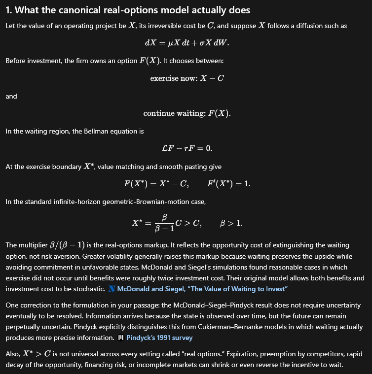


 Homework: talk to parents about a brokerage account, ahead of the July lab where students place their first real trades