
Summary and takeaways from Bridge Alternatives’ Portfolio Intuition (Link)
Intuition Test
Assume:
- Your current portfolio has 5% return and 15% volatility for a Sharpe ratio of .33
- You want to allocate 10% of your portfolio to a prospective asset
- You want to maximize the Sharpe ratio of the resulting portfolio
Choose between A1 and A2
| A1 | A2 | |
| Return | 4.00% | 4.00% |
| Volatility | 7.96% | 46.04% |
| Correlation | -.20 | -.20 |
Unsurprisingly, most people prefer A1 since it has the same attributes as A2 with 1/6 the risk.
Now let’s run the numbers
Expected return of the new portfolio is the same whether we choose A1 or A2:

Volatility of the new portfolio if we choose A1:

Sharpe ratio of original portfolio = .33
Sharpe ratio when we add A1 = .049/.13363 or .3667
The Sharpe ratio improved by about 10%
Now what is the Sharpe ratio if we add A2 instead of A1.
First, we must compute the volatility. Go ahead, plug and chug…

That’s right, the volatility is the same!
The volatility of the new portfolio is the same whether we add A1 or A2 which means the new combined portfolio has the same improvement to Sharpe whether we add A1 or A2. This is true despite A2 having a far worse Sharpe than A1! It is counterintuitive because portfolio math and the role of correlation is not intuitive.
To see why, look at the formula for portfolio volatility:
![]()
Let’s zoom in on the last 2 terms which come from adding the second asset:
Plot of change in overall portfolio volatility vs volatility of prospective asset (A1 or A2)

As we increase the asset’s risk, the first term grows exponentially, and the second term shrinks linearly (remember, the correlation is negative). It turns out that, at least temporarily, the shrinking effect from the negative correlation outweighs the exponential term.
There are 2 observations to note once you are done reeling from the bizarre impact of correlation.
- When adding a negatively correlated asset to a portfolio its risk must be incredibly high before it starts to degrade the Sharpe ratio of the final portfolio.
- Notice how, at least until we hit the vertex, if we move from left to right, representing an increase in risk, we’re actually reducing return. Put differently, if we added risk and didn’t reduce return we’d deliver more than a 10% improvement; risk has a positive payoff here, which is very cool. There is a significant range where we are reducing the prospective assets’ Sharpe and actually reducing the volatility of the new portfolio.
More Preference Tests
| B1 | B2 | C1 | C2 | D1 | D2 | |
| Return | 10.54% | 3.57% | 9.33% | 6.50% | 6.43% | -2.64% |
| Volatility | 20.00% | 20.00% | 27.50% | 12.50% | 10.00% | 40.00% |
| Correlation | .80 | -.20 | .40 | .40 | .50 | -.60 |
Most people agree:
- B1 was slightly preferred to B2. For the same risk, B1 delivers much more return, though B2’s correlation is better.
- C2 was preferred. It’s Sharpe is higher (about 0.52 versus about 0.34).
- D1 was preferred to D2. D1’s Sharpe ratio is much higher. D2’s return is negative
The punchline, of course, is that every one of these assets improves the Sharpe of the portfolio by the same 10%. Your intuition would tell you would prefer a portfolio in the upper left green box since those assets have the best Sharpe (risk/reward), so it is probably uncomfortable to learn that the final portfolio is mathematically indifferent to all of these assets.

Correlation Is The Key
Here’s the same plot relating these equivalent portfolios by their respective correlations

As the correlation drops (corresponding to lines of “cooler” coloring), less return is required to deliver the same 10% improvement!
While Sharpe ratios are “mentally portable”, they are shockingly incomplete without being tied to correlation. To create a compact formula which links Sharpe ratios with correlation, it is helpful to view indifference curves.
Indifference Curves
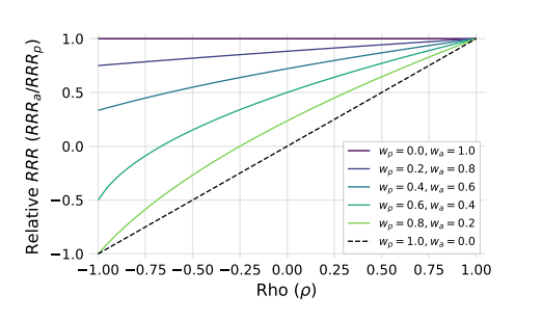
RRRa = Sharp Ratio of prospective asset
RRRb = Sharp Ratio of original portfolio
If Relative RRR > 1 the Sharpe of the prospective asset is greater than the Sharpe ratio of the original portfolio
The indifference curve represents an equivalent tradeoff between Sharpe ratio and correlation for various mixing weights. For example, the light green line assumes you will allocate 20% of the original portfolio to the prospective asset.
Observations
- As the weight allocated to the asset increases (the lines move upward, from green to purple), the asset must be more performant in order to do no harm; it must be better relative to the portfolio. Put differently, as the role played by the asset increases, more is required of it, and that sounds about right.
- A less performant asset, ie one with a worse Sharpe ratio than the original portfolio can compensate with low or negative correlations
Getting Practical
The investor’s natural question when evaluating a new asset or investment is:
“What is required from an asset (in terms of return, risk and correlation) in order to add value to my portfolio?”
With math that can be verified in the paper’s appendix we find a very handy identity:

This equality describes what’s required, in an absolute bare-minimum mathematical sense, of a prospective asset in order to do no harm.
How to use it
For a given prospective Sharpe ratio, you very simply compute the maximum correlation the new asset can have to be accretive to the portfolio. For example, if the prospective asset has a Sharpe ratio of .10 and the original portfolio has a Sharp ratio of .40 then the prospective asset requires correlation no greater than .25 (ie .10/.40).
For a given correlation, you can compute the minimum required Sharpe ratio of the new asset to improve the portfolio. If the correlation is .80 and the original portfolio has a Sharpe ratio of .70 then the prospective asset must have a Sharpe ratio of at least .56 (ie .80 x .70).
Insights and Caveats
- Correlation is best understood as a sort of performance hurdle. For assets exhibiting low correlation, less is required of their standalone performance (i.e. return over risk), all else equal.
- Prospective assets with a Sharpe ratio greater than the original portfolio are always additive.
- If you happen to find a truly zero-correlation asset it will be additive as long as it has positive returns. And as we saw with asset D2, a negative Sharpe Ratio asset can be additive if it has a negative correlation!
- This cannot be used to somehow rank prospective assets. It can only serve as a binary filter: yes or no. This might feel like a real limitation. Sharpe ratios are absolutely rankable. They are measurements of the same unit (risk). But as we’ve shown in this paper, those rankings are not indicative of their true value within the context of a portfolio. Making decisions based only on return and risk is like ranking runners based on their times without asking how far they ran. It doesn’t make sense. If you take away one thing from this paper, this should be it!
My Own Conclusions
- Correlations make portfolio math extremely unintuitive.
- Negative and low correlations can make poor or losing stand-alone investments great additions to a portfolio. The implications for the diversifying power of low or negative-yielding assets are significant. Bonds, cash, commodities, gold.
- Highly volatile assets with a negative correlation are tamed and even subtractive to the total risk of a portfolio.
- While the importance of low or negatively correlated assets is well known it’s possible it remains underappreciated.
Further reading
Breaking The Market’s outstanding post Optimal Portfolios For Two Assets
You will learn:
- How to mix assets by comparing their geometric returns.
- Correlation’s effect on portfolio construction is not linear.
- The closer correlations are to 1 the more they impact the recommended mix.
- Negative correlations are deeply valuable in portfolio construction, adding to the long term return. Positive correlations are harmful, limiting the benefit of diversification.
- The mixing range for the geometric returns is the combination of each asset’s variance, expanded or contracted based on the correlation between the two assets.
- Negative correlation is wonderful.
Tool
You can save your own copy here
You can also play with the numbers directly below
If you use options to hedge or invest, check out the moontower.ai option trading analytics platform